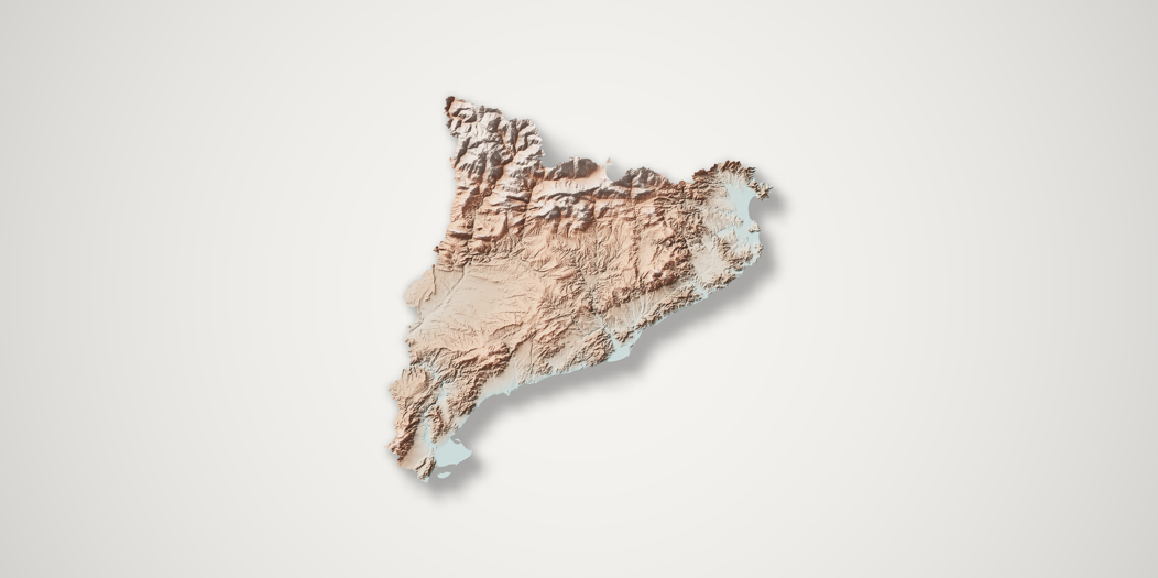
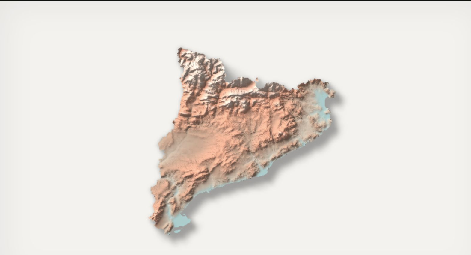
Engineering an orbitable cartographic height-field renderer: numerically refined intersections when settled, a rasterised proxy in motion, and terrain-space visibility shared by both.
I've always been a fan of relief maps and everytime I saw one of those shared online I wanted to implement a tool that generate them. During my 2026 summer holidays I thought I could do it while at the same time writing a WebGPU renderer from scratch. Estrat is the result.
This doc you are reading will, hopefully, guide you through what the tool does. You'll see there are a bunch of decisions to take to make the result great while also being performant. It will also be a way to remember how I implemented all this when I look back at it.
Without further ado, let me try to convey what a wonderful journey it is to go from height data to a rendered relief map.
Isaac
Pass 01 · InputsCPU / DATA REGISTRATION
Putting every input on the same grid
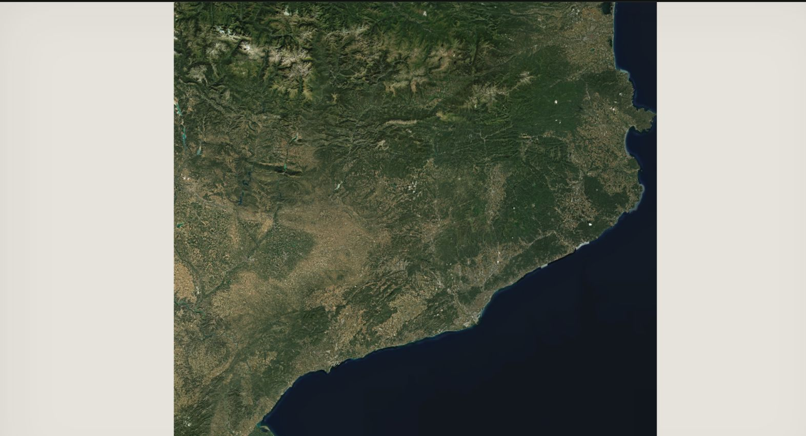
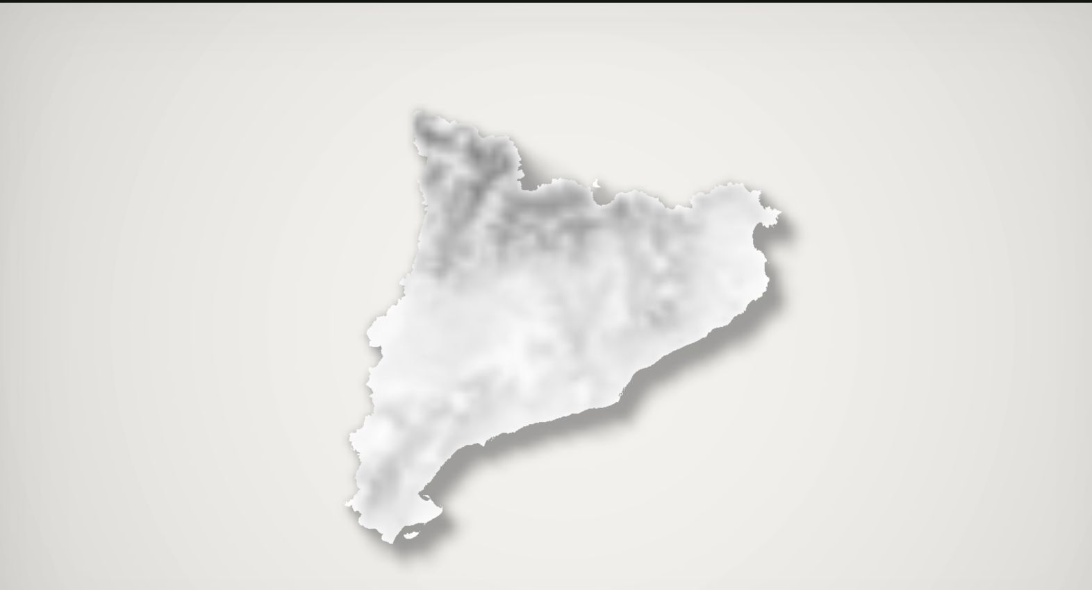
Once the selected region is chosen in the app, it is enclosed in a bounding box that becomes the output grid. For each cell of that grid, Estrat computes its position in the Web Mercator tile grid. It then uses each of those geographic positions to sample the elevation and style tiles and the rasterized boundary.
The elevation tiles use Terrarium RGB encoding, which the CPU decodes with the following formula per each pixel and normalises it
The source tiles are sampled into a shared destination grid; the coverage field is generated directly in that same grid.
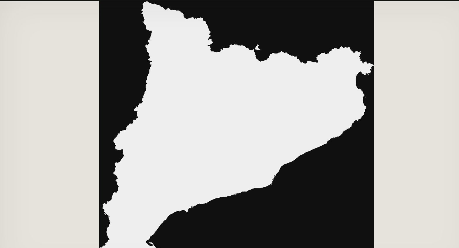
The boundary polygon is rasterised with an even-odd fill which gives us a binary coverage texture. A binary edge doesn't give good results because it creates an abrubt jumpt at the boundary which would result in rendering artifacts, so we turn it into a signed distance field by running a two-pass chamfer transform twice. On each transform, feature pixels start at distance 0 and every other pixel starts at Infinity. A forward, left-to-right/top-to-bottom, scan and a backward, right-to-left/bottom-to-top, scan then relaxes those values at cost 1 on cardinal neighbours and cost √2 at diagonal ones.
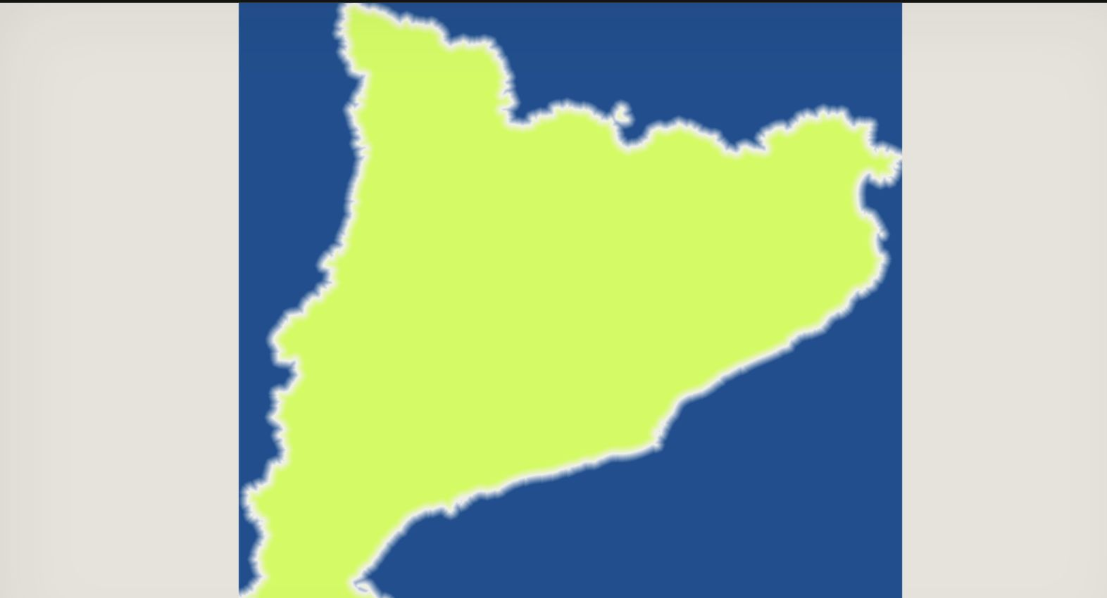
The first transform allows us to compute the distance to the nearest inside pixel. The second one measures the distance to the nearest outside pixel. For interior pixels we then keep the distance to the outside and for exterior pixels the negative distance to the inside:
Signed coverage distance
SDF(p) =  distance to outside, p inside
       −distance to inside,  p outside
Interior values are positive, exterior values are negative, and the zero contour lies between the two sides of the rasterised boundary.
This results in an approximate Euclidean distance, not a perfect geometric SDF. Its main job is to provide a stable sign and a useful contour that can be tested during ray traversal.
The signed-distance image replaces the binary edge with a graded field whose zero contour is the geographic boundary.
After that Estrat finds sea-level pixels that touch the raster edge or the outside of the selected polygon and uses a flood algorithm to remove ocean-connected sea-level cells without removing enclosed lakes.
Pass 02 · Terrain fieldsCPU / FILTERING
One DEM, two frequencies
Estrat builds two elevation textures from the elevation source: a macro field and a detail field.
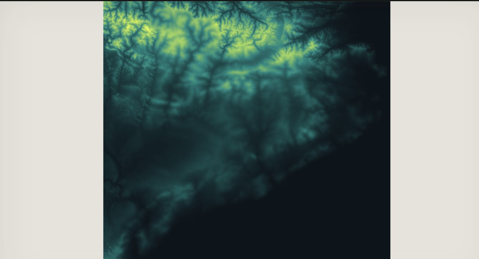
For the macro field we repeat a mask-aware separable blur pair three times to remove isolated DEM noise and preserve larger landforms. We then mix that with 15% of the source to avoid the result becoming completely flat. This becomes the authoritative surface for silhouettes, intersections and long shadows.
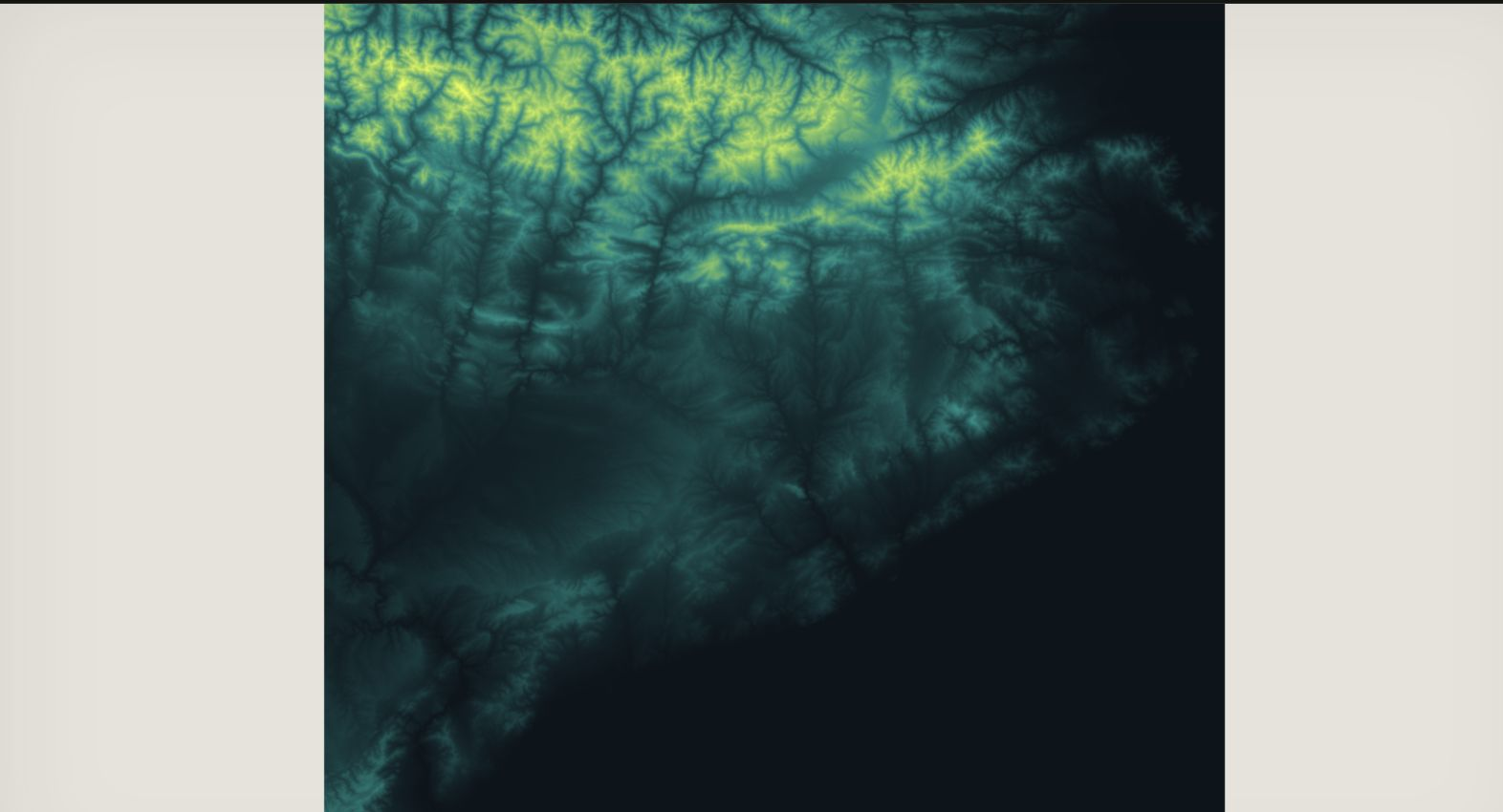
For the detail field we use two separable blur pairs using a 1-2-1 filter, creating a lightly smoothed detail field used for normals, short horizons, lowland cavities and elevation tint.
macro geometrydifferential detail
two height texturesone surface, two uses
Macro geometry controls where the surface is; detail controls how that surface is read.
Separating these frequencies keeps a noisy one-pixel DEM feature from becoming a spike or a kilometre-long shadow while preserving small structures in flat areas.
Pass 03 · Coverage and coordinatesGPU / WORLD SPACE
Turning texture samples into a height field
The CPU maps the selected area ground dimensions into a centered right-handed world, computing the aspect ratio from physical kilometers to avoid the view being distorted by longitude shrinking with latitude. Estrat then converts the world x,y to UV coordinates and samples the macro field as H(x,y).
Instead of just sampling the nearest pixel, Estrat loads the four surrounding values, interpolates across the top and bottom pairs and then interpolates between those two results. This bilinear lookup gives the ray marcher a continuous heigh function instead of pixel values that look like an staircase. The same kind of lookup is performed when sampling the signed-distance coverage field.
The macro field and the signed-distance coverage field answer different questions. The height texture says how high the surface is at a given position while the signed distance field says wether that position belongs to the selected area or not and how close it is to the edge. Having those two allows Estrat to stop treating the terrain as valid on boundaries during ray traversal to avoid creating vertical faces.
For an open relief, the implicit surface is simply:
Surface function
F(P) = P.z − H(P.x, P.y)
A point is on the terrain when its world height equals the interpolated DEM height at that horizontal position.
binary masksigned distanceheight field
Coverage and height remain separate fields: the SDF decides where terrain exists; H decides its elevation.Pass 04 · Primary visibilityGPU / FRAGMENT SHADER
Casting one ray per pixel
Estrat draws a full-screen triangle and, for each fragment, it builds an orthographic ray from yaw, pitch and distance values. Ray origins are backed away from the exaggerated relief to avoid tall peaks being behind the camera plane.
Given the previously defined surface function F(P) and the parametrical equation of a ray, P(t), what we need to do condenses to:
Ray / height-field intersection
find t where F(P(t)) = 0
Positive values are above the terrain; negative values are below it. The shader is looking for the first visible sign change along the ray.
Before sampling the DEM, the shader intersects the ray with the terrain’s axis-aligned bounding box using the slab method. This produces an entry and exit distance, tmin and tmax. Ray marching starts at max(tmin, 0) and stops at tmax with rays that miss the box returning immediately.
On ordinary rays, Estrat uses an adaptive advance. Given the current point, the shader measures the vertical separation |F(P)|, multiplies it by a conservative heuristic constant, and clamps the result between a minimum and maximum step. When the ray is far from the surface, this moves quickly. When the ray is near the surface, it takes shorter steps. The minimum prevents a nearly tangent ray from not moving while the maximum limits how many terrain cells the ray can cross in one advance.
Readers will notice this is not sphere tracing. That's a deliberate choice. |F(P)| gives us the vertical height, not the Euclidean distance to the surface and, since an oblique ray can travel a long horizontal distance while changing very little in z, using the raw separation as the step length could jump over narrow ridges. To avoid that, we conservatively allow a small number of texels per jump. Even when the vertical gap suggests a large step, this forces the ray to evaluate the terrain regularly enough that it's less likely to skip narrow ridges or valleys between samples.
After advancing along the ray, we check for a change in value signs, which means the surface lies between those two samples. Once a bracket is found, we keep refining via a fixed number of bisection steps. The final hit is the midpoint of the remaining interval, which is then used for normals, material and lightning.
Steps along a line. Notice how the distance between steps gets smaller the closer it is to the terrain.
Notice in the image above, that when the ray is far above the terrain, the height difference is large, so the next evaluation can be farther away. When the ray approaches the surface, the height shrinks, evaluating the height field more frequently, allowing us to buy precision near the place that matters without spending the same cost at every step.
Pass 05 · LightingGPU / COMPUTE + FRAGMENT SHADERS
Lighting the hit
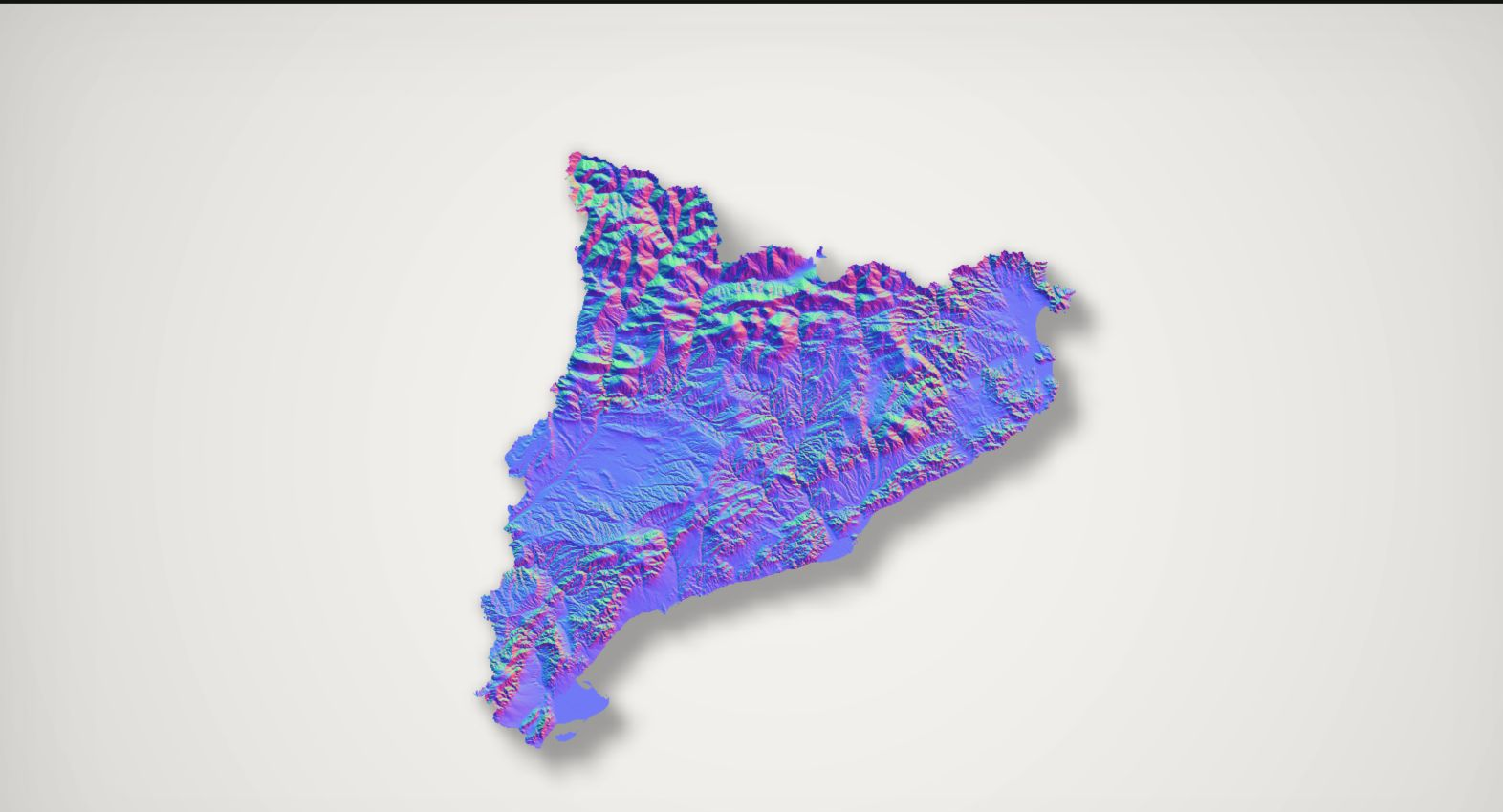
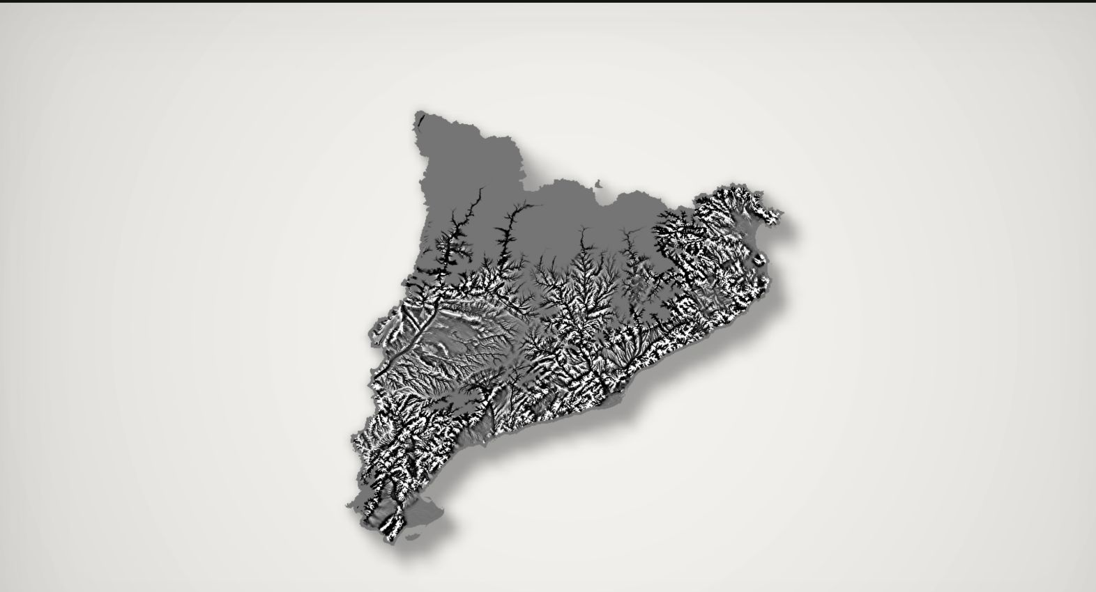
For any hit point, the shader samples the detail field on either side of the point and forms a scale-aware central difference to compute the normal. While the macro field defines the hit, the detail field supplies the local orientation.
macro height0.5N + 0.5
normal encodingR = east/west slopeG = north/south slopeB = up
Actual settled surfaceCentral differences
Central differences are symmetric. The normal map turns orientation into colour: horizontal components occupy red and green, upward direction blue.
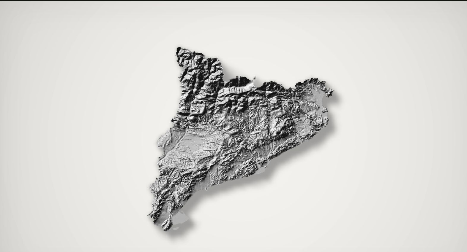
Lambert's cosine law is used to compute the direct light. A slope facing the sun must receive more direct light while a slope turning away receives less. Light azimuth and altitude are used to produce the unit light vector L.
material albedosurface orientationLambert N·L
Colour + orientationNo ambient terms
Lambert lighting immediately gives form, but it has no cast shadow and knows nothing about the surrounding sky.
After computing the direct light, Estrat uses a compute pass that fills a 384x384 world-space atlas with three values: Terrain sun visibility, which answers if the sunlight can reach the terrain surface, receiver sun visibility, which answers if the sunlight can reach the background, and a broad sky openess value, which tells how much of the surrounding sky is visibile from the terrain.
384x384 was chosen because it gives us ~145.5k cells, enough resolution for broad terrain shadows and horizons, while also being divisible by the 8x8 compute workgroup size.
orientationterrain visibilityreceiver visibility
Sun visibility is cached in terrain space, so it does not move when the camera orbits.
In order to make real valleys receive less of the sky than open plains, Estrat probes eight azimuthal horizons around every lighting-atlas cell. For each azimuth, twelve samples are placed at fixed distances. The shader then compares the height difference on each of those distances to the horizontal distance and retains the maximum positive slope. Computing the atan of that value converts the slope to a horizon angle. After that, normalising that angle against π/2 gives a simple openness fraction. Averaging the eight directions approximates the visible sky dome.
For each of eight plan-view directions, squared-distance probes search for the maximum elevation angle. A high ridge raises θmax and removes more of that directional slice of sky; the eight openness values are averaged.
B · 8×12 broad horizon6×5 local horizoncombined lighting
opennessdark = enclosedwhite = open hemisphere
Broad × local opennessTerrain-space
The maximum apparent slope in each direction reduces the visible sky. This is terrain-space, so camera motion cannot expose screen-space gaps.
The fragment shader adds six shorter, higher-resolution horizon probes from the detail field that are evaluated only for visible hits. While the compute atlas sees broad landforms, these higher-resolution horizon probes see local drainages without having to compute long horizons for every pixel.
Pyrenees · Lambert
central lowlands · local horizon
central lowlands · cavity
Crops from the same fixed frame expose the scale allocation: large gradients already describe the Pyrenees, while the plains depend on short-range horizon and residual signals.
Finally, the shader also evaluates a compact short-range obscurance heuristic. Six azimuths sample the detail field at three quadratically increasing distances. In each direction it first derives the slope of the tangent plane from the surface normal, then measures only terrain that rises above that plane. This conforms a view-independent contact-scale relief value that attenuates the sky term while leaving the direct sunlight alone.
Pass 06 · Materials and outputGPU / FRAGMENT SHADER
Applying cartographic colour
The hit's color is either sampled imagery, a solid colour or an hypsometric ramp that uses real elevation stops. To increase the contrast in low-lands, a two-radius residual compares the detail field with nearby means, updating the material brightness to capture local structure after the macro field has been smoothed.
The shader then combines the following values to decide the final color:
Albedo: The base surface color before lighting.
Sky fill: A soft ambient light representing diffuse light from the surrounding sky.
Overhead fill: Additional small amount of light for upward-facing surfaces.
Lamber diffuse
Cached sun visibility: Reduces the direct sunlight where the terrain blocks the sun.
Local horizons: Horizon probes that measure the nearby enclosure making valleys and locally-surrounded areas darker.
Ambient occlusion: To darken small concavities.
Blinn-style highlight
A1 · local direct
A2 · + Vsun
A3 · + Vbroad
A4 · + Vlocal
A5 · + AO
A6 · + cavity = final
A strict cumulative ablation from local direct response to the complete terrain shading. Because the output transfer remains enabled, differences are perceptual contributions in the delivered image rather than raw linear-term magnitudes.
Before output, the shader also applies an ACES-like tone curve and adds a small noise to prevent banding on smooth gradients.
Pass 07 · PresentationMESH / RAY-CAST SWITCH
Using cheaper representations while moving
Estrat uses the same macro field twice:
During pointer movement, a 192x192 indexed grid samples it in a vertex shader and rasterises a low-resolution mesh. This gives the browser a fixed-function triangle setup instead of running a long intersection loop for every pixel.
When pointer movement ends, the renderer schedules an intermediate ray-cast frame and then a full one. The shadow atlas is reused for camera-only changes while terrain, exaggeration, sun direction and shadow softness invalidate it.
moving: 192² meshsettled: implicit rays
Both modes consume the same height field and camera model; only the visibility strategy changes.ResultFINAL IMAGE
What the renderer is really doing
The final relief is not the product of a single heroic rendering trick: aligned rasters, macro and detail fields, terrain-sky visibility, etc. are all accumulated to drive the final result.
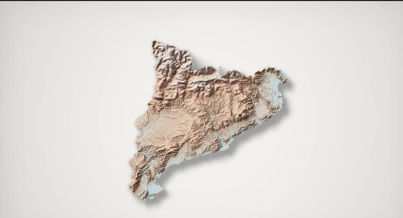
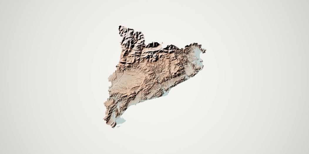
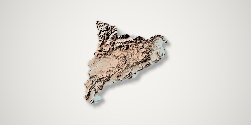
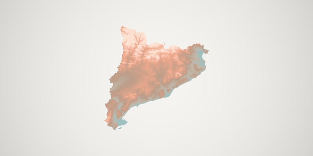
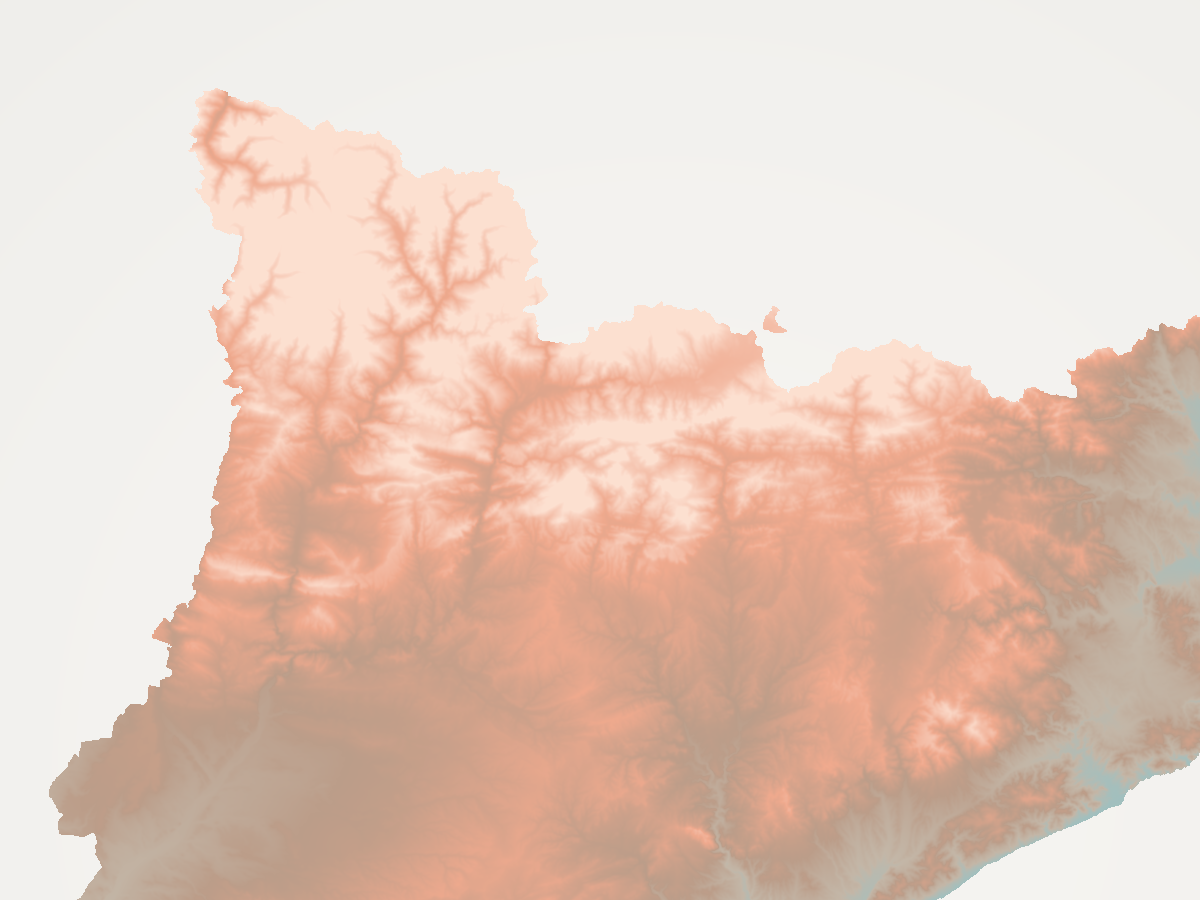
Following one Catalonia frame makes the dependencies visible. The northern Pyrenean ridge first appears as high scalar values, survives generalisation as broad geometry, acquires orientation through derivatives, blocks the finite north-west sun, closes the sky over neighbouring valleys and finally receives the upper-end of the adaptive tint. The low central and western lands barely change their silhouette, so they depend much more on detail normals, local horizons, cavity contrast and closely spaced low tint stops.
The sixteen development captures in pipeline order. Every tile comes from the same Catalunya terrain, camera, material and light.
The slider below allows you to see, on a fixed camera, how each step changes the final image.
Catalonia
Detail
1 / Albedo
The adaptive hypsometric material at the primary hit, before illumination.
Scrub from material input through Lambertian response, terrain shadow, broad and local sky visibility, local AO and lowland detail. Catalunya remains complete on the left.